Introduction

With the increasing trend of digitization in the last two decades, hard-copy documents have increasingly been uploaded onto databases for a variety of uses. Whether in the medical field, financial sector or in research circles, the process of digitization has been curbed only by the difficulty of the problem of automated reading of handwritten language on hard-copy papers. Though there are existing models and programs to allow this process, our group thought it would be an exceptional learning experience and quite fun to make our own, given a dataset that we have found and the resources given to us in the course, and through research.

Note: Proposal Modification

Originally, our project proposal focused on handwriting generation by giving a sample of handwriting and text to be written in that sampled handwriting; however, after further exploration into the problem, we realized many of the models to achieve such tasks were overly complicated and hard to replicate. Some of these models include conditional Generative Adversarial Networks and complicated LSTM-Attention Layer-MDN lego-like models. This is why we decided to instead reverse the problem and detect the text within handwriting. We had this change approved by a TA.

Problem Definition

This project aims to simplify potential hassle caused by trying to recognize and transfer written data to online format by creating a model which takes handwritten input and translate it to text format. Formally, the problem is a classification problem where given a series of handwritten strokes, the matching characters should be produced. This will be done by individually classifying letters. Effectively, the problem simplifies to a classification task where given an image of a character, to output the actual character in its ascii format.

Data Collection

The dataset comes from Kaggle and is called A-Z Handwritten Alphabets in .csv format. The dataset is a subset of the NIST dataset. It consists of a series of approximately 370,000 28 by 28 pixel grayscale images of alphabets with their according labels. Before applying any models on the data, we made sure to shuffle the dataset, as it was ordered based on ascii-ordering to ensure the training and testing sets had non-skewed distributions of characters. We also performed slight rotations on the data to ensure that our model would work on various types of characters in different orientations. In addition, due to the fact that the dataset was exceedingly large (encountering issues with RAM), we only used 100,000 samples of the dataset with an 80:20 training-testing split.

Scaling and PCA

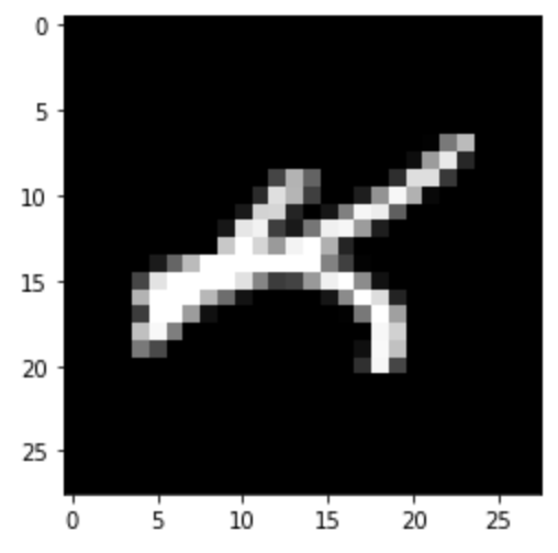
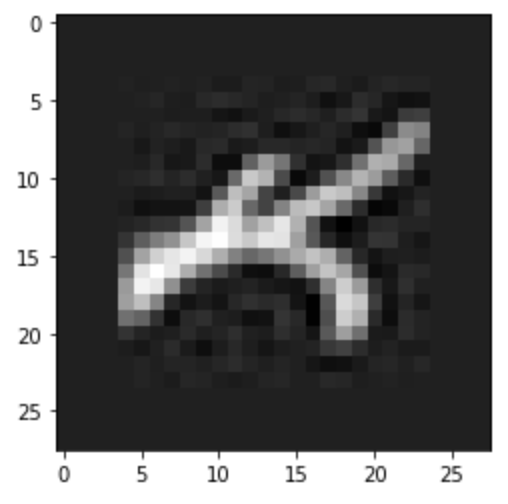
Furthermore, before feeding any data to a model, we ensured to perform dimensionality reduction by using standard scaling techniques and PCA with a retained variance of 0.98. For this, we used the python library scikit-learn. The images were practically the same (disregarding scaling) visually, though instead of each datapoint containing 784 features, the datapoint used 192 features. An example image, and the recovered image (with the scaling still applied) are shown below.

Methods

In order to perform the classification task defined above, we used two methods thus far: Mini-Batch K-Means and Convolutional Neural Networks. To implement both models we used common python packages like numpy, pandas, sklearn, and keras among others.

Mini-batch K-Means

Mini-batch K-Means is a variant of K-Means clustering that speeds up K-Means clustering by performing the reassignment and update steps on random samples of the original dataset. In turn, mini-batch K-Means tends to be quite faster at the cost of minor performance errors.

Although K-Means is typically an unsupervised learning technique, we added a final cluster-label matching procedure at the end of the algorithm to effectively convert into a supervised learning technique. After mini-batch K-Means produces each of its clusters, for each cluster, we looped through each datapoint, retrieved its corresponding training label, and assigned the cluster to the label most commonly present in the cluster. A basic code snippet highlights the procedure below.

kmean_labels = kmeans.labels_ #list of data points associated with a cluster index
mapping = {}  # (key, val) -->  (cluster_idx, label)

for i in range(len(kmean_labels)):
    k_label = kmean_labels[i]
    if k_label in mapping:
        mapping[k_label][train_labels[i]] += 1
    else:
        mapping[val] = [0 for i in range(26)]
        mapping[val][train_labels[i]] += 1

        for key in dic:
            mapping[key] = np.argmax(mapping[key]) #assigning cluster to max label count

Results and Discussion

To find the optimal number of clusters, we used the elbow method. Because K-Means is non-deterministic, we ran K-Means 10 times everytime for each number of clusters used to ensure we got a reasonably good elbow curve. Below is our results.

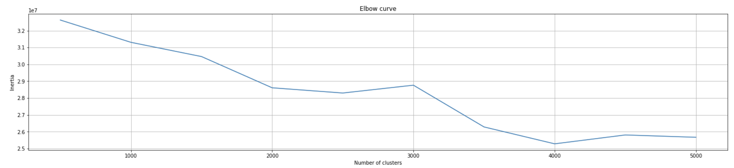
Evidently, at around 4000 clusters, the model performs the best. The inertia on the y-axis is simply another way to represent the distortion score: sum of squared distances for each point to its assigned cluster center.

As a precaution, we measured the accuracy for K-Means at various number of clusters to ensure that we didn’t have any oversight. Below are the results.

# of Clusters	Accuracy
26	48.53%
1000	79.84%
3000	85.3%
4000	84.179%

Although the elbow method suggested 4000 clusters would be the optimum number, it seems the highest accuracy of the cluster amounts tested about was 85.3% at 3000 clusters. This is not surprising because K-Means is non-deterministic meaning there may be some error in the elbow-method graph generated above (although we tried to reduce that by running K-Means multiple times).

85.3% is quite astounding performance for K-Means considering the fact that some of the images in the dataset were rotated quite significantly. Generally, one wouldn’t expect the algorithm to pick up on such rotations as K-Means uses a basic euclidean distance approach to measure similarity. It is very likely that there were “mini-clusters” which contained subclasses of each label. For example, one cluster may have contained the letter “A” but rotated 15% degrees to the left only, whereas another may have contained the letter “A” upright. In this sense, K-Means was able to detect spatial relationships by creating enough clusters to classify these spatial relationships.

Naturally, we hypothesize that if we were to used the normal variant of K-Means or Gaussian Mixture Model, we probably could have achieved higher accuracies. The reason why we chose not to use those models is to reduce training times, but more importantly, because we wanted to use clustering as a baseline for more complex and traidtional supervised models like convolutional neural networks.

Convolutional Neural Network

For the convolutional neural network (which from here on will be abbreviated as CNN), we tried many different architectures, loss functions, and optimizers, with various success and landed upon one architecture that was quite frankly surreal. This architecture was inspired by several models used on the MNIST dataset (handwritten digits) on Kaggle.

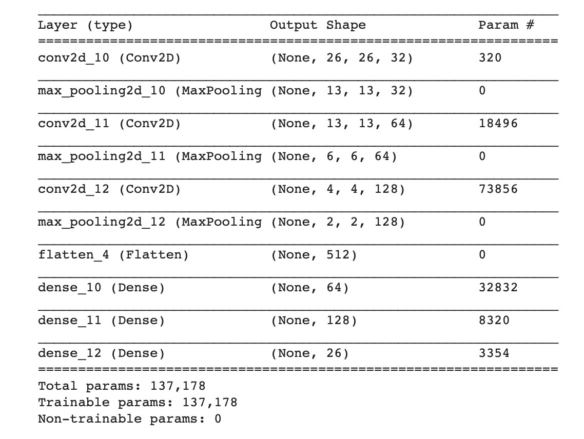
The model architecture is summarized in the image below.

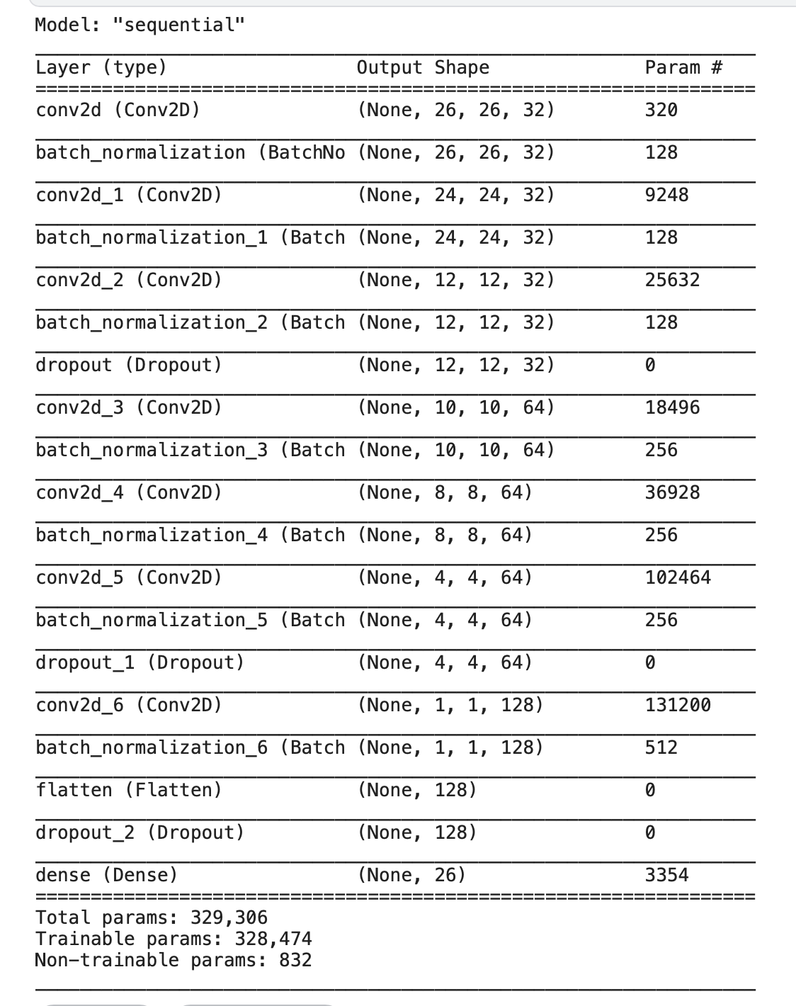
There are several things to point out about how this model is formed. One important factor is that it doesn’t rely on the data being compressed using dimensionality reduction beforehand. For the convolutional neural network, we decided to leave this out as we found it unnecessary given that the images being passed in are quite low resolution anyways, and that lowering the resolution further might make the filters act weirdly. Furthermore, for the same reason we chose not use max pooling (or average pooling) simply because the images were low resolution anyways and it didn’t seem to have any significant effect on the model (except adding more operations, at least for this model).

Our model is rather deep as it convolves hierarchically over the images. We found that around 300,000 parameters was a good number to learn most spatial relationships between the pixels. We included dropout and batch normalization layers after reading some Kaggle notebooks about how large models like this can easily overfit. The dropout layers effectively act as a form of regularization and the batch normalization layers make the model more stable and more importantly, quicker (training time took ~20 minutes for 10 epochs). We use cross-categorical entropy as our loss function inspired by what we learned in class about binary cross-entropy for classification and the popular Adam optimizer (as it seemed to perform better). ReLU was our primary loss function for speed reasons, and we used one-hot encoding to represent our labels.

Results and Discussion

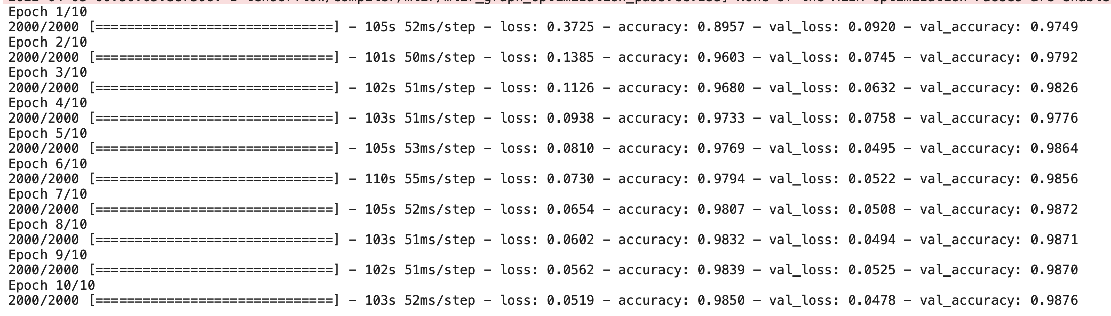
We trained over 10 epochs, as after that the model began to overfit and because the training time was getting exceedingly hard to work with. Below is a graphical representation of our training accuracy and validation accuracy over time. We used 20% of our training data as validation data to see if the model would generalize well. This is also how we tuned our Dropout layer hyperparameters.

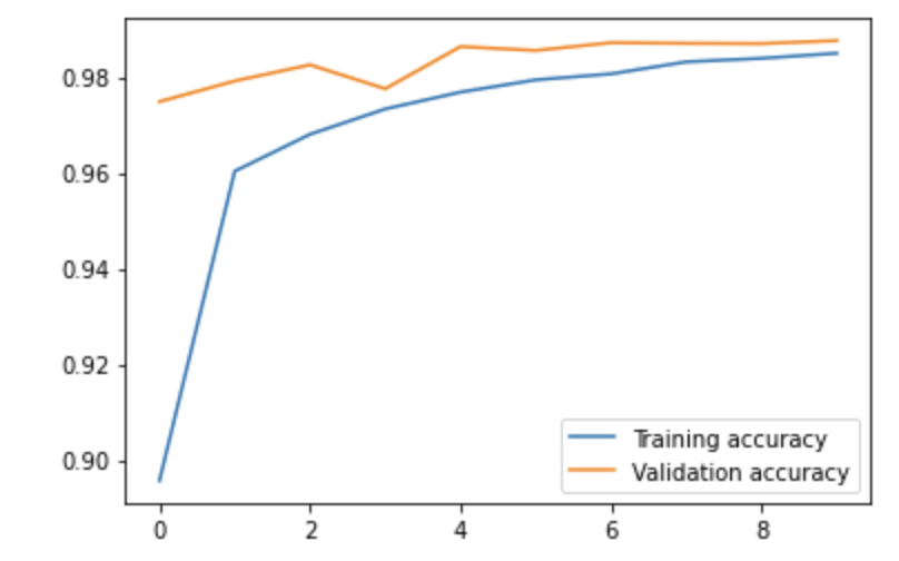
Interestingly enough, the validation accuracy was higher than our training accuracy. However, this is due to the fact we used a Dropout layer which zeros out certain features during training time but not during testing/validation time. Below is a summary of the training phase.

Once we tried the model on our testing set, we saw an accuracy of 98.75%. This was quite spectacular! This is most likely because our model is quite deep and involves a set of filters that grow through the model to capture many spatial features. K-Means, being a simple model, can’t really capture these relationships and does not have enough parameters to model such complexity.

Convolutional Neural Network with Max Pooling

Evidently, CNN’s seemed to perform at a relatively high accuracy (>98%), however, we wanted to test whether max pooling was necessary. In our previous model, we speculated that with batch normalization, max pooling wouldn’t be as necessary for quicker computations. With this model, we wanted to simplify the model by using less parameters to hopefully achieve comparable results to the CNN without max pooling. Much of the architecture changed significantly compared to the CNN used without max pooling. While we still use the same activation function for ‘relu’ and same loss function, as compared to the previous CNN, we focused on removing convolutional layers and adding more dense neural network layers. This included the addition of 2 more dense layers sandwiching our original dense layer in the original CNN model. We then proceeded to remove all the batch normalization and dropout layers, and instead fully relied on max pooling. We played around with the model and found that we could remove many of the convolutional layers doing the “thinking” by adding more dense layers. This also greatly reduced the number of parameters by approximately ~200,000. The architecture is summarized below.

Results and Discussion

When training this model, we saw an accuracy of 98.30% which was very comparable to the previous model, despite removing almost 200,000. Evidently, max pooling seems to be a more effective way for neural networks at least in the context of this problem to learn quickly about handwritten characters than a series of batch normalizations and dropouts combined with convolutional layers. We speculate this is because of the additional dense layers as well which can do more “feature engineering” with pooled features and take full advantage of max pooling. We also believe that if that max pooling were to be added to our previous model without the dense layers, it probably wouldn’t fair as well. This model could potentially be improved by introducing more regularization like dropout like our previous model, and more hyperparameter tuning.

Overall Results and Discussion

Evidently, the convolutional neural network without max pooling thus far has had amazing performance on the task, giving an accuracy of 98.75%, whereas using mini-batch K-Means has given an accuracy of 85.3%. It is important to note that this type of performance most likely has to do with the low resolution of each of images in the dataset (28 by 28 pixels). Having a lower resolution means there are less potential relationships to capture as opposed to an image that is (1000 by 1000 pixels) and thus easier to analyze for a model. It is important to note that these percentages can probably be increased by doing more fine-tuning and potentially using ensemble techniques that take into account the opinions of multiple models.

Below are the confusion matrices for both models.

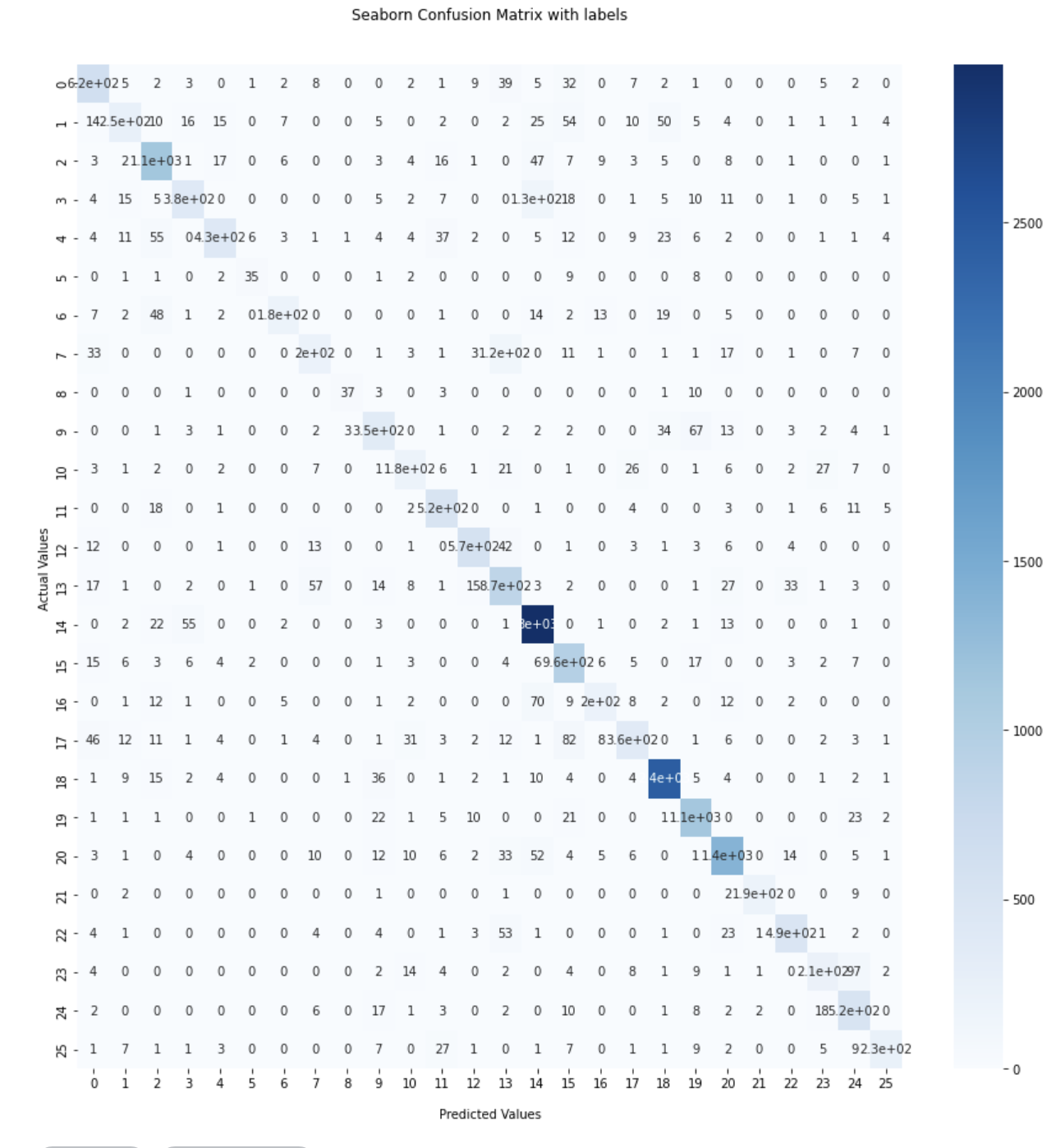
Evidently, the CNN without max pooling performed better as shown in the confusion matrices, but more importantly it seems that both models did well overall as indiciated by how sporadic the misclassified labels are. It seems that K-Means managed to confuse letters like “D” and “P” as well as “H” and “M” whereas the CNN picked up on that much better.

The CNN with max pooling also performed rather spectacularly at 98.30%. We decided to use this model to see if we could optimize our architecture and hyperparameters to achieve better accuracy. While we weren’t able to achieve a better accuracy with this model, it was evident that this model was the most practical in terms of deployability in the real world due to how simple this model is. By shaving off about 200,000 parameters, the model had much quicker training times, and in the real world, would be much more effective on larger training sets. The model still suffers from overfitting as indiciated by the validation losses being somewhat lower than training losses, and the lack of any mechanism to prevent overfitting (like dropout, etc). In the future, this model could be improved by combining the architecture with the more performant network that uses batch normalization and dropout. K-Means, while being an interesting way to approach this problem, falls too short to be used in the real world.

Conclusions

Convolutional neural networks seem to be the most effective at solving this classification problem due to their massive complexity, spatial feature engineering, and non-linearity. K-Means performed decently, however, this may be due to the simplicity of the dataset used, and in the real world, K-Means may not perform so admirably. While, one of our models was the most performant, we believe that CNN without max pooling should not be deployed in the real world for transferring files from text format to digital format. We believe this because we created a CNN that used a much simpler architecture (max pooling) with quicker training times that can be adapted more quickly as more training data comes in to achieve better accuracies.

At approximately 98% accuracy, our best models performed rather well. To improve these accuracies in the future, we propose purposely engineering certain features that can help distinguish confusing characters as shown by our confusion matrix before like “D” and “P”. These features would be very informative to the neural network and could be provided directly to the dense layers instead of through the convolutional layers where these features may be lost.

We also believe our models are ready to be used in the present. We hope to release some of our models to the public on Kaggle for both educational purposes and potential commerical purposes. We also intend to potentially create a web app that performs handwritten recognition to ascii conversions.

Dataset

https://www.kaggle.com/datasets/sachinpatel21/az-handwritten-alphabets-in-csv-format

References

1. https://ai.stackexchange.com/questions/20680/should-neural-nets-be-deeper-the-more-complex-the-learning-problem-is
2. https://www.kaggle.com/code/abdulmeral/10-models-for-clustering/notebook
3. https://nanonets.com/blog/handwritten-character-recognition/
4. https://paperswithcode.com/task/handwriting-recognition
5. https://medium.com/geekculture/max-pooling-why-use-it-and-its-advantages-5807a0190459